Forecasting with a variational quantum algorithm — inside Qortex's Mil'HaQ Fest win
How team Qortex used a variational quantum algorithm — a parametrized circuit trained in a hybrid quantum-classical loop and run on IBM's ibm_quebec processor — to forecast a financial time series, and took first place in the Quantum Machine Learning track at Mila's Mil'HaQ Fest 2025.
At Mil’HaQ Fest 2025, the Qiskit Fall Fest hackathon hosted by Mila — Quebec AI Institute, team Qortex took first place in the Quantum Machine Learning track. The challenge: forecast the next steps of a financial time series — a grid of interest-rate values indexed by tenor and maturity. Our answer was a variational quantum algorithm (VQA): a parametrized quantum circuit whose rotation angles are trained, the same way a neural network’s weights are, to minimize a forecasting error. This post walks through how it works and how we ran it on real quantum hardware.
The full project lives in the Qortex repository; the forecasting model is in src/ and the hardware run is captured in the ibm_quebec execution notebook.
The idea: a hybrid quantum-classical loop
A variational quantum algorithm splits the work between two machines. A quantum computer holds a parametrized circuit with three parts — an encoding stage that loads the input data as rotation angles, a trainable ansatz of parametrized gates, and a measurement stage that reads expectation values back out. A classical computer takes those measurements, evaluates a cost function, and uses a classical optimizer to nudge the circuit’s parameters in the direction that lowers the cost. Repeat until it converges.
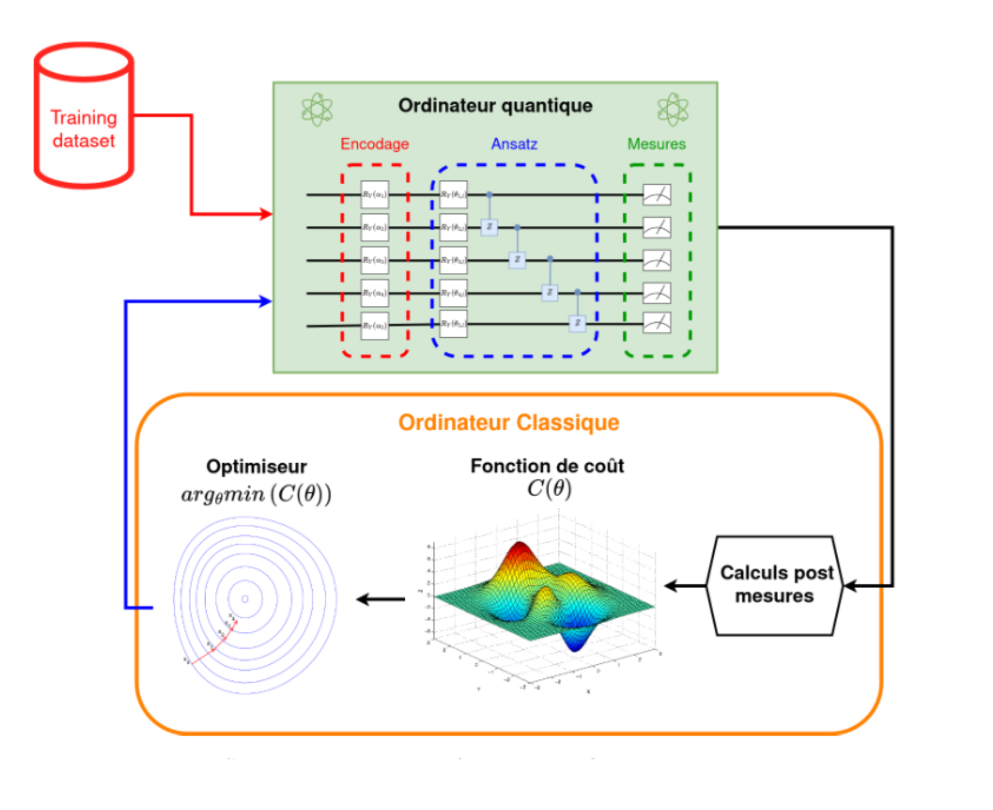
That feedback loop is the whole trick: the quantum circuit is a feature map we can tune, and the classical optimizer does the tuning.
The circuit: encoding plus a trainable ansatz
Our circuit runs on six qubits. The input — a short window of the time series, reduced to six numbers — is encoded once as a layer of RY rotations. After that come reps repeated blocks, each a layer of trainable RY(θ) rotations followed by a cascade of CZ gates that entangles neighbouring qubits. The θ angles are the only things that get trained.
from qiskit import QuantumCircuit
from qiskit.circuit import Parameter

def make_feature_circuit(n=6, reps=4):
    qc = QuantumCircuit(n)

    # 1) Encode the 6 input features once, as RY rotation angles
    data_params = []
    for q in range(n):
        p = Parameter(f"data_{q}")
        qc.ry(p, q)
        data_params.append(p)

    # 2) Trainable blocks: a layer of RY(theta) + a CZ entangling cascade
    theta_params = []
    for r in range(reps):
        row = []
        for q in range(n):
            t = Parameter(f"theta_{r}_{q}")
            qc.ry(t, q)
            row.append(t)
        theta_params.append(row)

        for q in range(n - 1):
            qc.cz(q, q + 1)

    return qc, data_params, theta_params
With reps=4 the ansatz looks like this — one data-encoding layer, then four trainable RY(θ) layers interleaved with the entangling cascade:
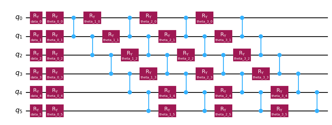
data_*) followed by four trainable RY(θ) layers (theta_r_q), each chained to the next by a staircase of two-qubit entangling gates.Reading the circuit out as features
To turn the circuit into a layer we can put inside a model, we measure the expectation value of Z on each qubit — six numbers, ⟨Z₀⟩ … ⟨Z₅⟩. On the simulator this is exact via the statevector; the layer is just a torch.nn.Module whose theta is a trainable parameter tensor.
class QiskitObsLayer(nn.Module):
    def __init__(self, n=6, reps=4):
        super().__init__()
        self.n, self.reps = n, reps
        self.template, self.data_params, self.theta_params = make_feature_circuit(n, reps)
        self.theta = nn.Parameter(0.01 * torch.randn(reps, n))   # trainable angles
        # One Z observable per qubit
        self.obs = [
            SparsePauliOp.from_list([("I"*i + "Z" + "I"*(n-i-1), 1.0)])
            for i in range(n)
        ]

    def forward(self, x):
        out = []
        for b in range(x.shape[0]):
            angles = x[b].reshape(6).tolist()
            assign = {self.data_params[q]: float(angles[q]) for q in range(self.n)}
            for r in range(self.reps):
                for q in range(self.n):
                    assign[self.theta_params[r][q]] = float(self.theta[r, q].detach())

            state = Statevector.from_instruction(self.template.assign_parameters(assign))
            out.append([float(state.expectation_value(o).real) for o in self.obs])
        return torch.tensor(out, dtype=torch.float32)
The full model is that quantum feature map followed by a small classical linear head, trained end-to-end with Adam and an MSE loss:
class Model(nn.Module):
    def __init__(self):
        super().__init__()
        self.q = QiskitObsLayer()   # quantum feature map -> 6 expectation values
        self.fc = nn.Linear(6, 6)   # classical read-out head
    def forward(self, x):
        return self.fc(self.q(x)).view(-1, 3, 2)
Before any of this, the raw rate grid is compressed to two principal components with PCA, then sliced into sliding windows — three time steps in, the next three predicted. At inference the model runs autoregressively: each prediction is fed back in to forecast the step after it, and PCA’s inverse transform maps the result back to the original rate grid.
Running it on ibm_quebec
The interesting part was moving off the simulator and onto a real device — IBM’s ibm_quebec processor. Two things change. First, you can no longer read ⟨Z⟩ exactly; you sample the circuit and reconstruct each expectation value from measurement counts. Second, real qubits decohere while they sit idle, so we transpile at the highest optimization level and add a dynamical decoupling schedule — periodic X pulses that refocus idle qubits and claw back fidelity.
from qiskit_ibm_runtime import QiskitRuntimeService, SamplerV2 as Sampler
from qiskit.transpiler.preset_passmanagers import generate_preset_pass_manager
from qiskit.transpiler import PassManager
from qiskit.circuit.library import XGate
from qiskit_ibm_runtime.transpiler.passes.scheduling import (
    ALAPScheduleAnalysis, PadDynamicalDecoupling, DynamicCircuitInstructionDurations,
)

service = QiskitRuntimeService()
backend = service.backend("ibm_quebec")

durations = DynamicCircuitInstructionDurations.from_backend(backend=backend)
pm = generate_preset_pass_manager(target=backend.target, optimization_level=3)

# Dynamical decoupling: pad idle windows with a sequence of X gates
pm.scheduling = PassManager([
    ALAPScheduleAnalysis(durations=durations),
    PadDynamicalDecoupling(
        durations=durations,
        dd_sequences=[XGate()] * 8,
        pulse_alignment=16,
    ),
])
The expectation values then come from the sampled bitstrings instead of the statevector — |0⟩ counts as +1, |1⟩ as −1, weighted by how often each was measured:
sampler = Sampler(backend)
job = sampler.run(transpiled_circuits, shots=1024)
result = job.result()

# Reconstruct <Z_i> from the measured bitstring statistics
for i, pub_result in enumerate(result):
    counts = pub_result.data.meas.get_counts()
    total = sum(counts.values())
    expectation = 0.0
    for bitstring, count in counts.items():
        bits = [int(b) for b in bitstring[::-1]]        # qiskit little-endian
        expectation += (1 - 2 * bits[i]) * count / total  # |0> -> +1, |1> -> -1
This was the most hardware-hungry stretch of the weekend. Qortex leaned on ibm_quebec harder than anyone else at the event — across all the teams, roughly 80% of every job submitted to the device over the hackathon was ours, as Ismael iterated on the transpilation passes and the dynamical-decoupling schedule to keep the on-device expectation values close enough to the simulator’s for the model to keep learning.
The result
The forecasting VQA — trained in a hybrid loop, validated on the simulator, and executed end-to-end on ibm_quebec — earned team Qortex first place in the Quantum Machine Learning track at Mil’HaQ Fest 2025. Not bad for one weekend, six qubits, and a lot of dynamical decoupling.
Comments & corrections
If you have questions about this note, or you spot something we got wrong, please write to the author directly. We post addenda to articles when a correction is warranted.